Assessing the new class of d-i-d estimators
A replication
Dan Killian
DALL-E interpretation of my final preparation

Outline of presentation
- Background
- Problem
- Solutions
- Case study - MISTI
- Final thoughts
Bottom line up front
- In certain settings, beware the Two-Way Fixed Effects Estimator!
- Don’t conflate your modeling approach (TWFE) with your estimation strategy
- Examine the different groups created by differential timing
- Use event study designs
- Specify a fully flexible model (Two-way Mundlak)
- Background
- Problem
- Solutions
- Case study - MISTI
- Final thoughts
D-i-D has a long and storied history
- Ignaz Semmelweis - Let’s track mortality rates in two maternity wards, one staffed with midwives and the other with medical students (who were busy with cadavers)
![]()

D-i-D has a long and storied history
- John Snow: Let’s track cholera infection in two London neighborhoods, one with treated water and one without


D-i-D has a long and storied history
- Economists - Let’s steal repeated measures ANOVA from the statisticians!
“This estimator has been labeled the difference-in-differences estimator in the recent program evaluation literature, although it has a long history in analysis of variance.” [Wooldridge 2010]
Cross Validated: Difference in Difference vs repeated measures
So what is the canonical d-i-d setup?
\(y_{it}=\beta_0+\delta_{0,t}Post_t+\beta_{1,i}Treat_i+\delta_{1,it}Post_t*Treat_i+\epsilon_{it}\)
where..
\(\beta_0\) is the comparison group at baseline
\(\delta_0\) is the secular change from baseline to endline, unrelated to treatment
\(\beta_1\) is the difference between the treatment and comparison groups at baseline, and
\(\delta_1\) is the treatment effect, the interaction of treatment and time
Algebraically, \(\delta_0\) can be expressed as the difference between the pre/post difference in each of the treatment and comparison groups
\(\delta_1=\)
\((\bar{y}_{POST,TREAT}-\bar{y}_{PRE,TREAT})\)
\(-\)
\((\bar{y}_{POST,COMPARISON}-\bar{y}_{PRE,COMPARISON})\)
hence, difference-in-differences (d-i-d or DiD or DD)
Canonical d-i-d, 2x2
\(y_{it}=\beta_0+\delta_{0,t}Post_t+\beta_{1,i}Treat_i+\delta_{1,it}Post_t*Treat_i+\epsilon_{it}\)
| Pre | Post | Post - Pre | |
|---|---|---|---|
| Comparison | \(\beta_0\) | \(\beta_0+\delta_0\) | \(\delta_0\) |
| Treatment | \(\beta_0+\beta_1\) | \(\beta_0+\delta_0+\beta_1+\delta_1\) | \(\delta_0+\delta_1\) |
| Treatment - Comparison | \(\beta_1\) | \(\beta_1 + \delta_1\) | \(\delta_1\) |
How does the canonical d-i-d generalize to multiple time periods and/or groups?
When we generalize the two-period setup to multiple time periods and/or groups, we have the two-way fixed effect (TWFE) estimator
\(y_{it}=\alpha_i+\alpha_t+\beta^{DD}{it}+\epsilon_{it}\)
where..
\(\alpha_i\) are group fixed effects
\(\alpha_t\) are time fixed effects
\(B^{DD}_{it}\) indicates whether group i in period t is treated
TWFE is a workhorse in program evaluation
744 d-i-d studies across ten journals in finance and accounting, 2000-2019 [Baker 2022]
19 percent of all empirical articles published by the American Economic Review (AER) between 2010 and 2012 used TWFE [de Chaisemartin and D’Haultfoeuille 2020]
- Background
- Problem
- Solutions
- Case study - MISTI
- Final thoughts
But what is \(\beta^{DD}_{it}\) actually telling us?
For the canonical 2x2, we know exactly what we are estimating
For i groups and t time periods, we are getting some average of multiple 2x2s
But how does this work, exactly?
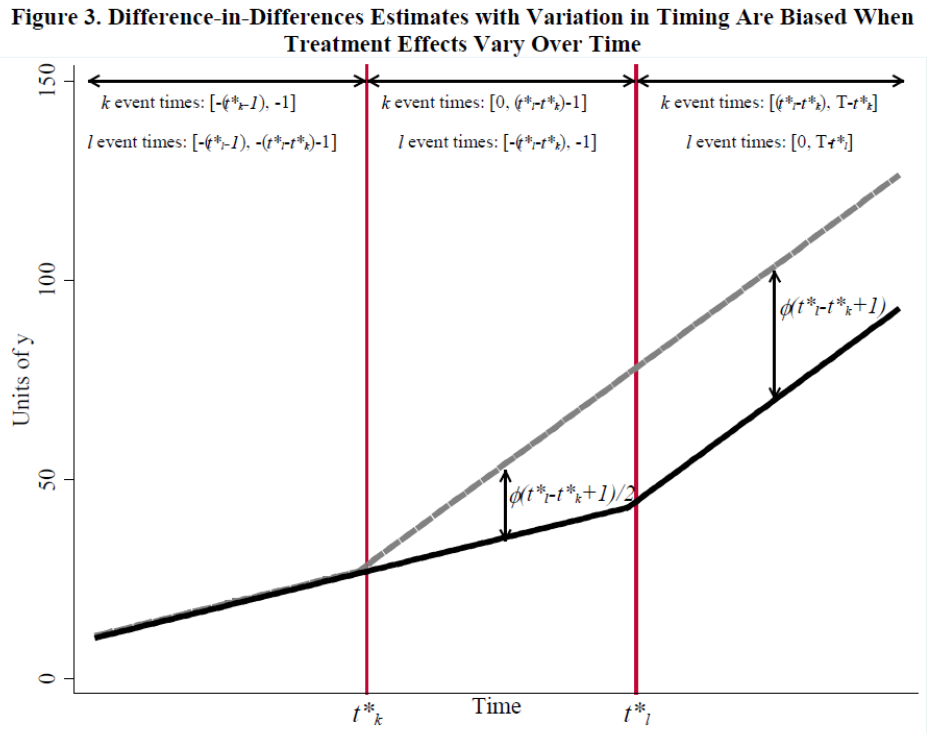
Goodman-Bacon (2021) decided to work it out
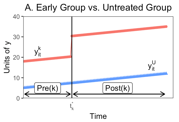
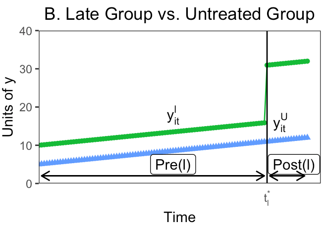
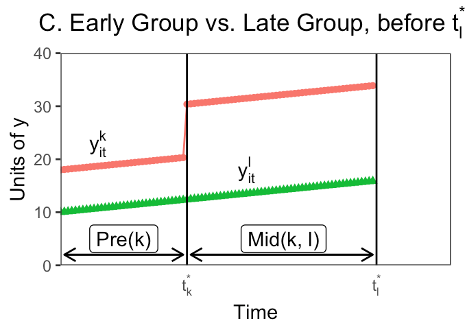
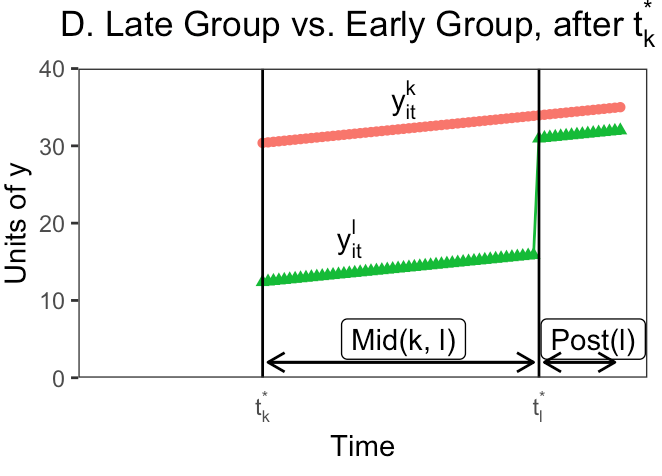
Let’s take a single step from two time periods to three, where treatment can be adopted at either t = 2 or t = 3
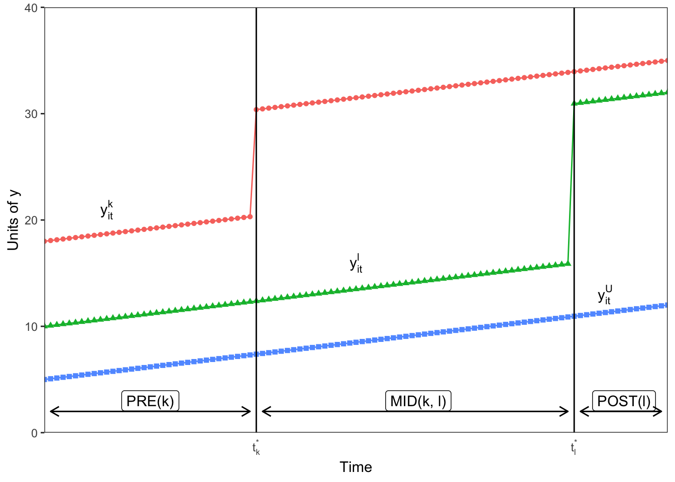
Any design with multiple treatment timings will have \(k^2\) groups, where k is the number of timings.
Where does this leave us?
- TWFE treats some data that is under treatment status as comparison!
- Not an issue under constant treatment effect
- stable unit treatment value (SUTVA)
- no variation in treatment effect for any reason
But TWFE fails under following conditions:
- different treatment groups have different treatment effects
- treatment effects are dynamic over post-treatment periods
- heterogeneous treatment effects across sub-groups within a treated group
An example of failure
- Background
- Problem
- Solutions
- Case study - MISTI
- Final thoughts
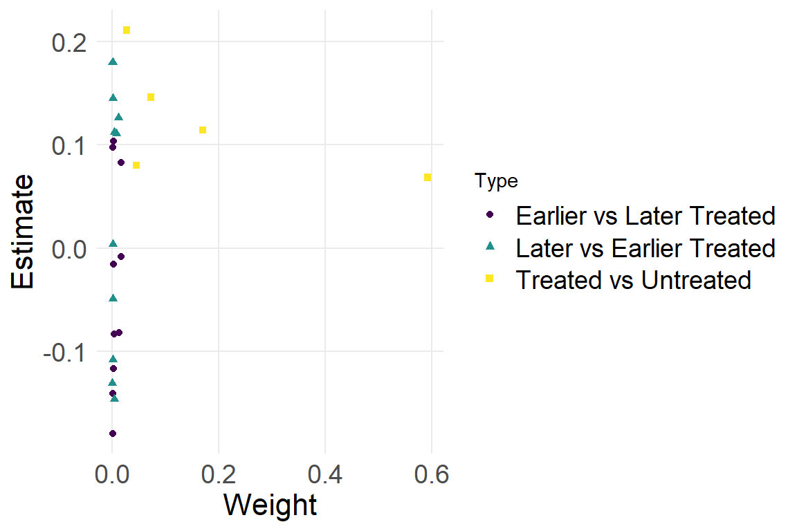
Diagnostic: the Bacon decomposition
- The Bacon decomposition will take a TWFE model and decompose it into the full array of 2x2 d-i-d cells used to construct the overall estimate
- The decomposition will also calculate the variance-weights used in regression to see which 2x2 cells are powering the overall estimate
| treated | untreated | estimate | weight | type |
|---|---|---|---|---|
| 2005 | 2006 | -0.08313 | 0.003405 | Earlier vs Later Treated |
| 2005 | 2007 | -0.11672 | 0.002095 | Earlier vs Later Treated |
| 2005 | 2008 | -0.14123 | 0.001571 | Earlier vs Later Treated |
| 2005 | 2009 | 0.09714 | 0.001048 | Earlier vs Later Treated |
| 2005 | 99999 | 0.08017 | 0.045569 | Treated vs Untreated |
| 2006 | 2005 | -0.14607 | 0.003405 | Later vs Earlier Treated |
| 2006 | 2007 | 0.08302 | 0.016342 | Earlier vs Later Treated |
| 2006 | 2008 | -0.00848 | 0.016342 | Earlier vs Later Treated |
| 2006 | 2009 | -0.08226 | 0.012256 | Earlier vs Later Treated |
| 2006 | 99999 | 0.06824 | 0.592395 | Treated vs Untreated |
| 2007 | 2005 | -0.10806 | 0.001676 | Later vs Earlier Treated |
| 2007 | 2006 | 0.12596 | 0.010895 | Later vs Earlier Treated |
| 2007 | 2008 | 0.10372 | 0.002933 | Earlier vs Later Treated |
| 2007 | 2009 | -0.01598 | 0.002933 | Earlier vs Later Treated |
| 2007 | 99999 | 0.11406 | 0.170124 | Treated vs Untreated |
| 2008 | 2005 | -0.04898 | 0.000943 | Later vs Earlier Treated |
| 2008 | 2006 | 0.11069 | 0.008171 | Later vs Earlier Treated |
| 2008 | 2007 | 0.14479 | 0.001257 | Later vs Earlier Treated |
| 2008 | 2009 | -0.17989 | 0.000838 | Earlier vs Later Treated |
| 2008 | 99999 | 0.14605 | 0.072910 | Treated vs Untreated |
| 2009 | 2005 | 0.17952 | 0.000419 | Later vs Earlier Treated |
| 2009 | 2006 | 0.11210 | 0.004085 | Later vs Earlier Treated |
| 2009 | 2007 | 0.00373 | 0.000838 | Later vs Earlier Treated |
| 2009 | 2008 | -0.13078 | 0.000210 | Later vs Earlier Treated |
| 2009 | 99999 | 0.21108 | 0.027341 | Treated vs Untreated |
Adjustment: new estimators
R packages for new d-i-d estimators
| Reference | R package | Description |
|---|---|---|
| Callaway Sant'Anna (2020) | did | Compare treatment only to never treated, or never-treated + not-yet-treated. Also propensity score weights with covariates. |
| Sun Abraham (2020) | fixest | NA |
| Chaisemartin D'Haultfoeuille (2020) | DIDmultiplegt | NA |
| Wooldridge (2021) | fixest | Dummies for all group, time, time-to-treat, time-since-treatment units |
- Background
- Problem
- Solutions
- Case study - MISTI
- Final thoughts
Measuring Impact of Stabilization Initiatives (MISTI)
Can small scale, community-driven development activities build local government legitimacy in a kinetic conflict-affected environment?
MISTI
- Village panel survey in five waves, Sep 2012 - Nov 2014
- ~5,000 villages surveyed across 130 districts and 23 provinces
- ~ 30,000 household interviews per wave
- 860 treated villages at any wave (17%)
- 355 villages surveyed in all five waves
- 85 villages treated (24%)

MISTI treatment timings
| Wave | Comparison villages | Treated villages | Treated villages (cumulative) |
|---|---|---|---|
| 1 | 355 | 0 | 0 |
| 2 | 341 | 14 | 14 |
| 3 | 322 | 19 | 33 |
| 4 | 302 | 20 | 53 |
| 5 | 270 | 32 | 85 |
Single-wave analysis
- Final reporting of MISTI relied on a series of single-wave estimations
| Measure | Wave 2-4 | Wave 2-5 | Wave 3-4 | Wave 4-5 | Wave 3-5 |
|---|---|---|---|---|---|
| Stability | 0.031 | 0.043 | 0.003 | -0.039 | -0.002 |
| Government Capacity | 0.044 | 0.054 | 0.032 | -0.038 | 0.007 |
| District Government Performance | 0.053 | 0.053 | 0.046 | -0.069 | -0.031 |
| District Government Satisfaction | 0.006 | -0.019 | 0.007 | 0.027 | 0.002 |
| Provincial Government Performance | 0.067 | 0.067 | 0.056 | -0.064 | 0.005 |
| Local Governance | 0.012 | 0.031 | 0.031 | -0.035 | 0.003 |
| DDA-CDC Performance | 0.000 | 0.035 | 0.034 | -0.064 | -0.015 |
| Local Leader Performance | 0.001 | 0.015 | -0.001 | 0.045 | 0.015 |
| Quality of Life | 0.039 | 0.016 | -0.003 | -0.012 | -0.027 |
| Resilience | 0.015 | 0.007 | 0.056 | -0.004 | 0.017 |
| Community Cohesion | -0.029 | -0.014 | -0.044 | 0.027 | 0.058 |
| Social Capital | -0.037 | -0.022 | -0.095 | 0.001 | 0.074 |
| Local Leader Satisfaction | 0.009 | 0.016 | 0.022 | 0.046 | 0.028 |
MISTI TWFE
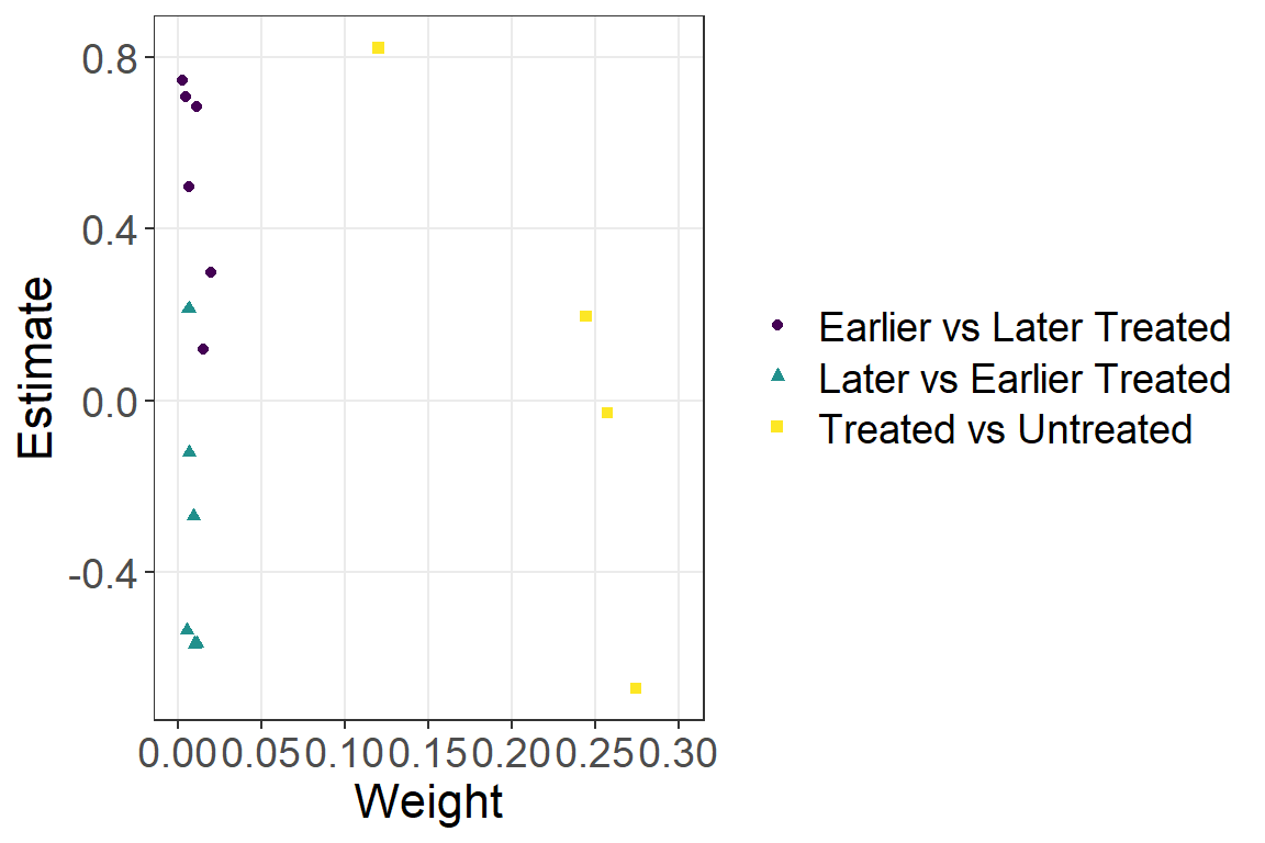
MISTI bacondecomp
| treated | untreated | estimate | weight | type |
|---|---|---|---|---|
| 2 | 3 | 0.7473 | 0.00211 | Earlier vs Later Treated |
| 2 | 4 | 0.7093 | 0.00444 | Earlier vs Later Treated |
| 2 | 5 | 0.6868 | 0.01066 | Earlier vs Later Treated |
| 2 | 99999 | 0.8232 | 0.11998 | Treated vs Untreated |
| 3 | 2 | -0.1216 | 0.00633 | Later vs Earlier Treated |
| 3 | 4 | 0.4973 | 0.00603 | Earlier vs Later Treated |
| 3 | 5 | 0.2976 | 0.01930 | Earlier vs Later Treated |
| 3 | 99999 | 0.1964 | 0.24425 | Treated vs Untreated |
| 4 | 2 | -0.2707 | 0.00889 | Later vs Earlier Treated |
| 4 | 3 | 0.2135 | 0.00603 | Later vs Earlier Treated |
| 4 | 5 | 0.1182 | 0.01524 | Earlier vs Later Treated |
| 4 | 99999 | -0.0291 | 0.25710 | Treated vs Untreated |
| 5 | 2 | -0.5680 | 0.01066 | Later vs Earlier Treated |
| 5 | 3 | -0.5686 | 0.00965 | Later vs Earlier Treated |
| 5 | 4 | -0.5375 | 0.00508 | Later vs Earlier Treated |
| 5 | 99999 | -0.6729 | 0.27424 | Treated vs Untreated |
Callaway and Sant’Anna (2020)
This estimation gives you multiple outcomes
- Treatment by treatment group
- An overall treatment effect
- Overall dynamic effects / event study
- Treatment effects by calendar time
Callaway and Sant’Anna replication
cal <- att_gt(yname="stab_std",
             tname="wave",
             idname="idname",
             gname="first.treat",
             xformla= ~ nsp + ln_dist,
             data=mistifull)
summary(cal)
Call:
att_gt(yname = "stab_std", tname = "wave", idname = "idname",
    gname = "first.treat", xformla = ~nsp + ln_dist, data = mistifull)

Reference: Callaway, Brantly and Pedro H.C. Sant'Anna.  "Difference-in-Differences with Multiple Time Periods." Journal of Econometrics, Vol. 225, No. 2, pp. 200-230, 2021. <https://doi.org/10.1016/j.jeconom.2020.12.001>, <https://arxiv.org/abs/1803.09015>

Group-Time Average Treatment Effects:
 Group Time ATT(g,t) Std. Error [95% Simult.  Conf. Band]
     2    2   0.4105      0.381       -0.6179       1.439
     2    3   0.9595      0.432       -0.2089       2.128
     2    4   1.2952      0.452        0.0734       2.517 *
     2    5   0.5136      0.460       -0.7298       1.757
     3    2  -0.2553      0.265       -0.9704       0.460
     3    3   0.3693      0.258       -0.3271       1.066
     3    4   0.3161      0.263       -0.3949       1.027
     3    5   0.2650      0.220       -0.3305       0.861
     4    2   0.1522      0.224       -0.4532       0.758
     4    3  -0.3197      0.263       -1.0308       0.391
     4    4   0.1823      0.274       -0.5590       0.923
     4    5   0.0491      0.259       -0.6500       0.748
     5    2   0.3244      0.203       -0.2243       0.873
     5    3  -0.1808      0.191       -0.6978       0.336
     5    4  -0.1153      0.170       -0.5752       0.344
     5    5  -0.5982      0.181       -1.0881      -0.108 *
---
Signif. codes: `*' confidence band does not cover 0

P-value for pre-test of parallel trends assumption:  0.46101
Control Group:  Never Treated,  Anticipation Periods:  0
Estimation Method:  Doubly Robust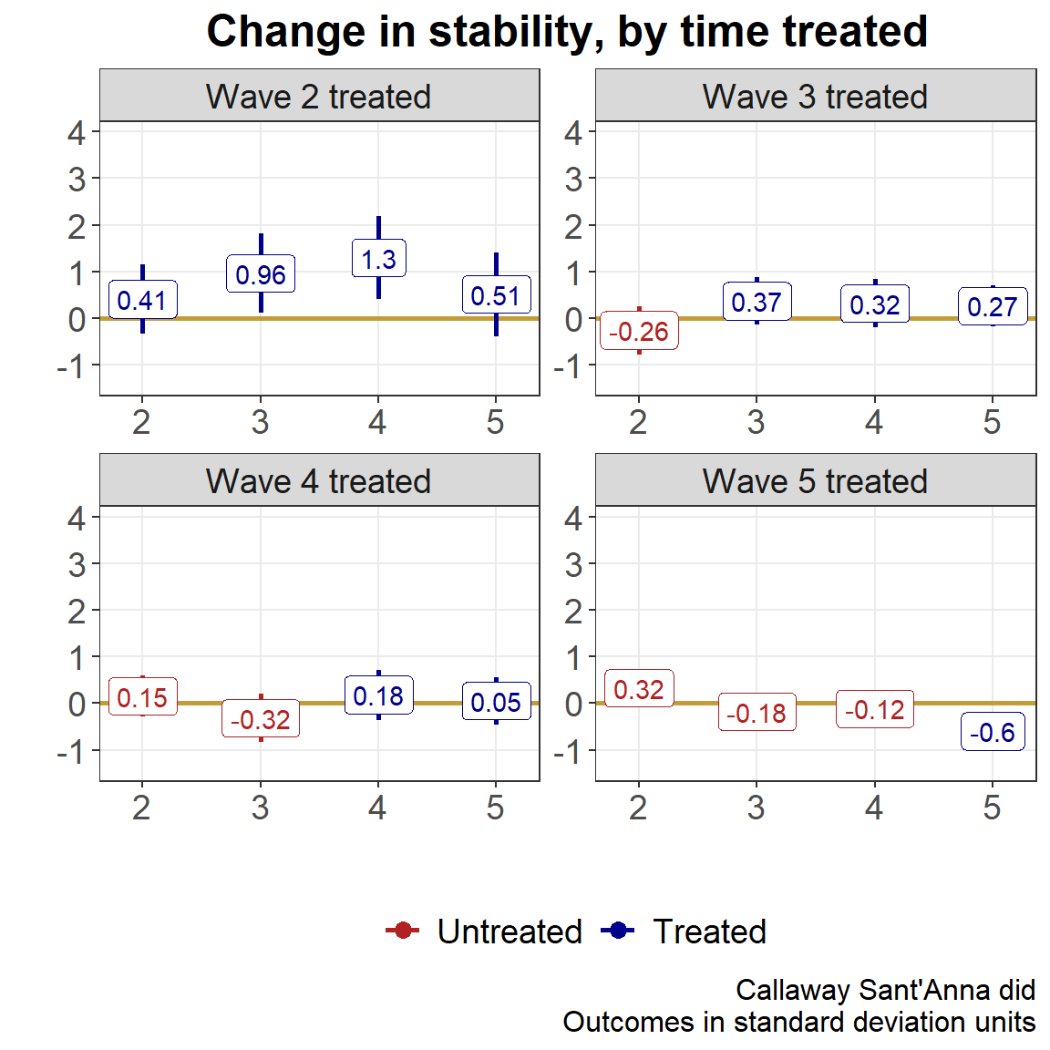
Call:
aggte(MP = cal, type = "simple")

Reference: Callaway, Brantly and Pedro H.C. Sant'Anna.  "Difference-in-Differences with Multiple Time Periods." Journal of Econometrics, Vol. 225, No. 2, pp. 200-230, 2021. <https://doi.org/10.1016/j.jeconom.2020.12.001>, <https://arxiv.org/abs/1803.09015>


  ATT    Std. Error     [ 95%  Conf. Int.]
 0.26          0.16    -0.0538       0.573


---
Signif. codes: `*' confidence band does not cover 0

Control Group:  Never Treated,  Anticipation Periods:  0
Estimation Method:  Doubly Robust
Call:
aggte(MP = cal, type = "dynamic")

Reference: Callaway, Brantly and Pedro H.C. Sant'Anna.  "Difference-in-Differences with Multiple Time Periods." Journal of Econometrics, Vol. 225, No. 2, pp. 200-230, 2021. <https://doi.org/10.1016/j.jeconom.2020.12.001>, <https://arxiv.org/abs/1803.09015>


Overall summary of ATT's based on event-study/dynamic aggregation:
   ATT    Std. Error     [ 95%  Conf. Int.]
 0.392         0.191     0.0172       0.767 *


Dynamic Effects:
 Event time Estimate Std. Error [95% Simult.  Conf. Band]
         -3   0.3244      0.214       -0.2291       0.878
         -2  -0.0527      0.136       -0.4048       0.299
         -1  -0.2104      0.123       -0.5282       0.107
          0  -0.0322      0.135       -0.3815       0.317
          1   0.3853      0.176       -0.0698       0.840
          2   0.7021      0.241        0.0771       1.327 *
          3   0.5136      0.488       -0.7498       1.777
---
Signif. codes: `*' confidence band does not cover 0

Control Group:  Never Treated,  Anticipation Periods:  0
Estimation Method:  Doubly Robust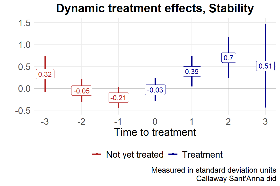
Call:
aggte(MP = cal, type = "group")

Reference: Callaway, Brantly and Pedro H.C. Sant'Anna.  "Difference-in-Differences with Multiple Time Periods." Journal of Econometrics, Vol. 225, No. 2, pp. 200-230, 2021. <https://doi.org/10.1016/j.jeconom.2020.12.001>, <https://arxiv.org/abs/1803.09015>


Overall summary of ATT's based on group/cohort aggregation:
    ATT    Std. Error     [ 95%  Conf. Int.]
 0.0037         0.116     -0.224       0.232


Group Effects:
 Group Estimate Std. Error [95% Simult.  Conf. Band]
     2    0.795      0.374       -0.0975       1.687
     3    0.317      0.200       -0.1587       0.792
     4    0.116      0.240       -0.4554       0.687
     5   -0.598      0.181       -1.0305      -0.166 *
---
Signif. codes: `*' confidence band does not cover 0

Control Group:  Never Treated,  Anticipation Periods:  0
Estimation Method:  Doubly Robust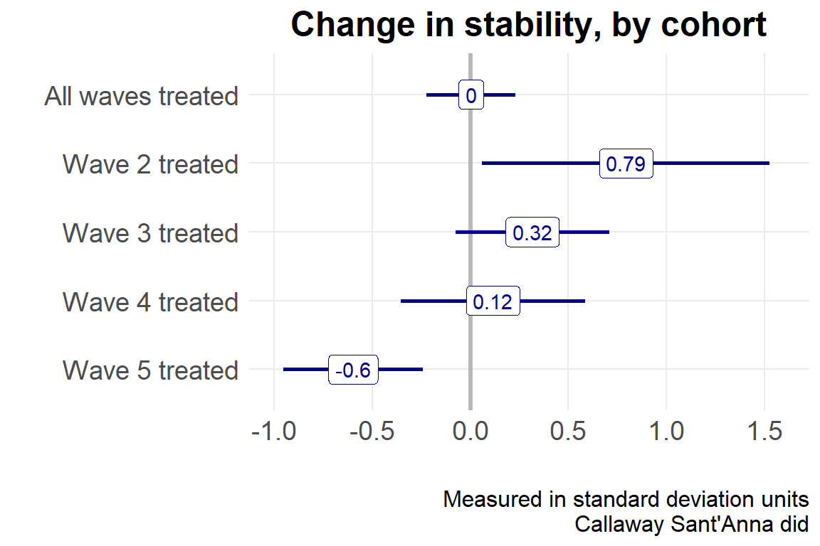
Call:
aggte(MP = cal, type = "calendar")

Reference: Callaway, Brantly and Pedro H.C. Sant'Anna.  "Difference-in-Differences with Multiple Time Periods." Journal of Econometrics, Vol. 225, No. 2, pp. 200-230, 2021. <https://doi.org/10.1016/j.jeconom.2020.12.001>, <https://arxiv.org/abs/1803.09015>


Overall summary of ATT's based on calendar time aggregation:
   ATT    Std. Error     [ 95%  Conf. Int.]
 0.371         0.179     0.0196       0.723 *


Time Effects:
 Time Estimate Std. Error [95% Simult.  Conf. Band]
    2   0.4105      0.389       -0.5214       1.342
    3   0.6197      0.245        0.0325       1.207 *
    4   0.5242      0.201        0.0432       1.005 *
    5  -0.0698      0.148       -0.4248       0.285
---
Signif. codes: `*' confidence band does not cover 0

Control Group:  Never Treated,  Anticipation Periods:  0
Estimation Method:  Doubly Robust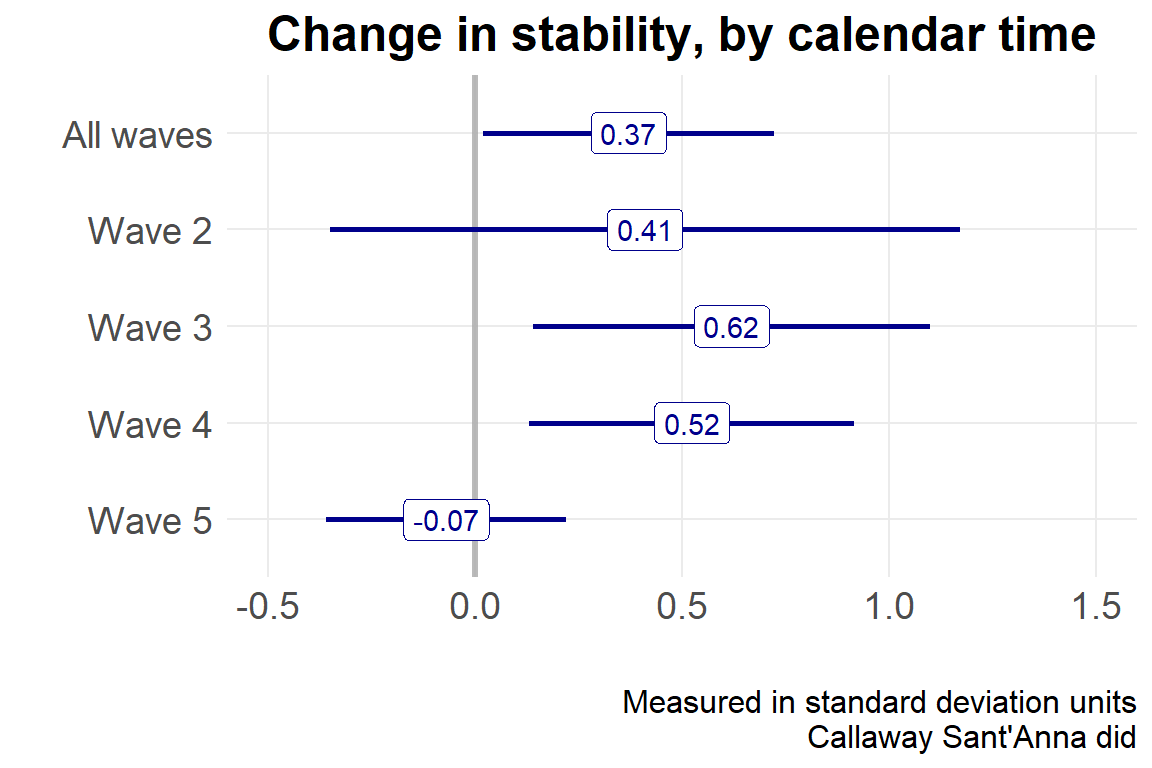
- Background
- Problem
- Solutions
- Case study - MISTI
- Final thoughts
What have we learned?
- In certain settings, two-way fixed effects estimation is biased in ways that we only recently came to realize
- We have to carefully think through the data generating process (logic modeling) for each individual setting
- As we get more granular data and ask deeper questions, econometric tools are starting to provide better insight into treatment dynamics
What should we do?
- For any two-way fixed effects setting, use the Bacon decomposition to diagnose any problems
- Use stacked d-i-d to remove problematic 2x2 cells, or apply any of the new estimators
- Go back to your old evaluations!!
THANK YOU!!
dkillian@msi-inc.com
Please evaluate this session!
The next slide shows two DALL-E narratives
How would you rate the quality of this session, where 1 reflects the scenario on the left, and 5 reflects the scenario on the right?