South Sudan

Resilience Panel Survey

Introduction

There are 613 records in this dataset.

Household structure

Sources of Income

Code

#include_graphics(here("output/viz/income sources 2.png"))

Code

inc2 <- read_csv(here("output/tables/Income sources.csv"),
                show_col_types=F)

inc_gt <- inc2 %>%
  dplyr::select(`Income source` = lab, Percent=mean) %>%
  mutate(Bar=Percent*100) %>%
  gt() %>%
  gt_plt_bar_pct(column=Bar, fill=usaid_blue, background=light_grey, scaled=T) %>%
  cols_width(3 ~ px(125)) %>%
  fmt_percent(2, decimals=0) %>%
  cols_label(Bar="")

inc_gt

Income source	Percent
Farm/crop production	90%
Wild bush sales	46%
Goat production/sales	31%
Fishing and sales	23%
Cattle production/sales	22%
Ag wage labor in village	20%
Petty trade own products	18%
Petty trade other products	15%
Food / cash safety net	14%
Salaried work	12%
Other self-employment non-ag	10%
Wage labor in village	8%
Sheep production/sales	8%
Honey production/sales	6%
Ag wage labor outside village	5%
Other self-employment ag	5%
Other	5%
Remittances	2%
Wage labor outside village	1%
Gifts/inheritance	1%
Rental of land/property	0%

Food Insecurity

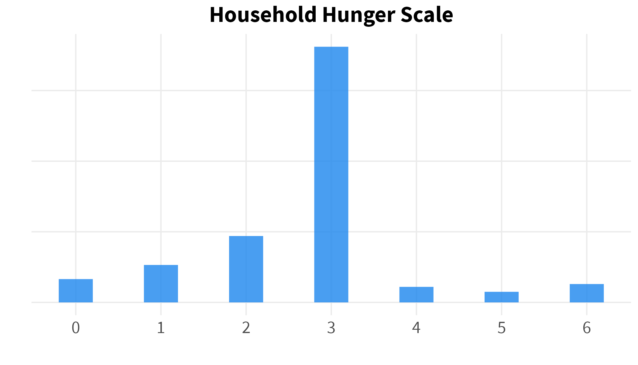
Household Hunger Scale

Items

Code

hhs <- read_csv(here("output/tables/Household hunger scale.csv"),
                show_col_types=F)

hhs_gt <- hhs %>%
  dplyr::select(1, Percent) %>%
  mutate(Bar=Percent*100) %>%
  gt() %>%
  gt_plt_bar_pct(column=Bar, fill=usaid_blue, background=light_grey, scaled=T) %>%
  cols_width(3 ~ px(125)) %>%
  fmt_percent(2, decimals=0) %>%
  cols_label(Bar="")

hhs_gt

In previous four weeks..	Percent
Lack of resources to get food	86%
Went to sleep hungry	89%
Whole day without eating	75%
Severe household hunger	10%

Scale frequencies

Code

include_graphics(here("output/viz/household hunger bar.png"))

By county

Code

hhs_sev_cnty <- read_csv(here("output/tables/hhs severe county.csv"),
                         show_col_types=F)

hhs_sev_cnty_gt <- hhs_sev_cnty %>%
  dplyr::select(county, hhs_severe) %>%
  mutate(Bar=hhs_severe*100) %>%
  gt() %>%
  gt_plt_bar_pct(column=Bar, fill=usaid_blue, background=light_grey, scaled=T) %>%
  cols_width(3 ~ px(125)) %>%
  fmt_percent(2, decimals=0) %>%
  cols_label(hhs_severe="Severe household hunger",
    Bar="")

hhs_sev_cnty_gt

county	Severe household hunger
Pibor	40%
Akobo	17%
Jur River	3%
Wau	2%
Budi	1%
Kapoeta North	0%

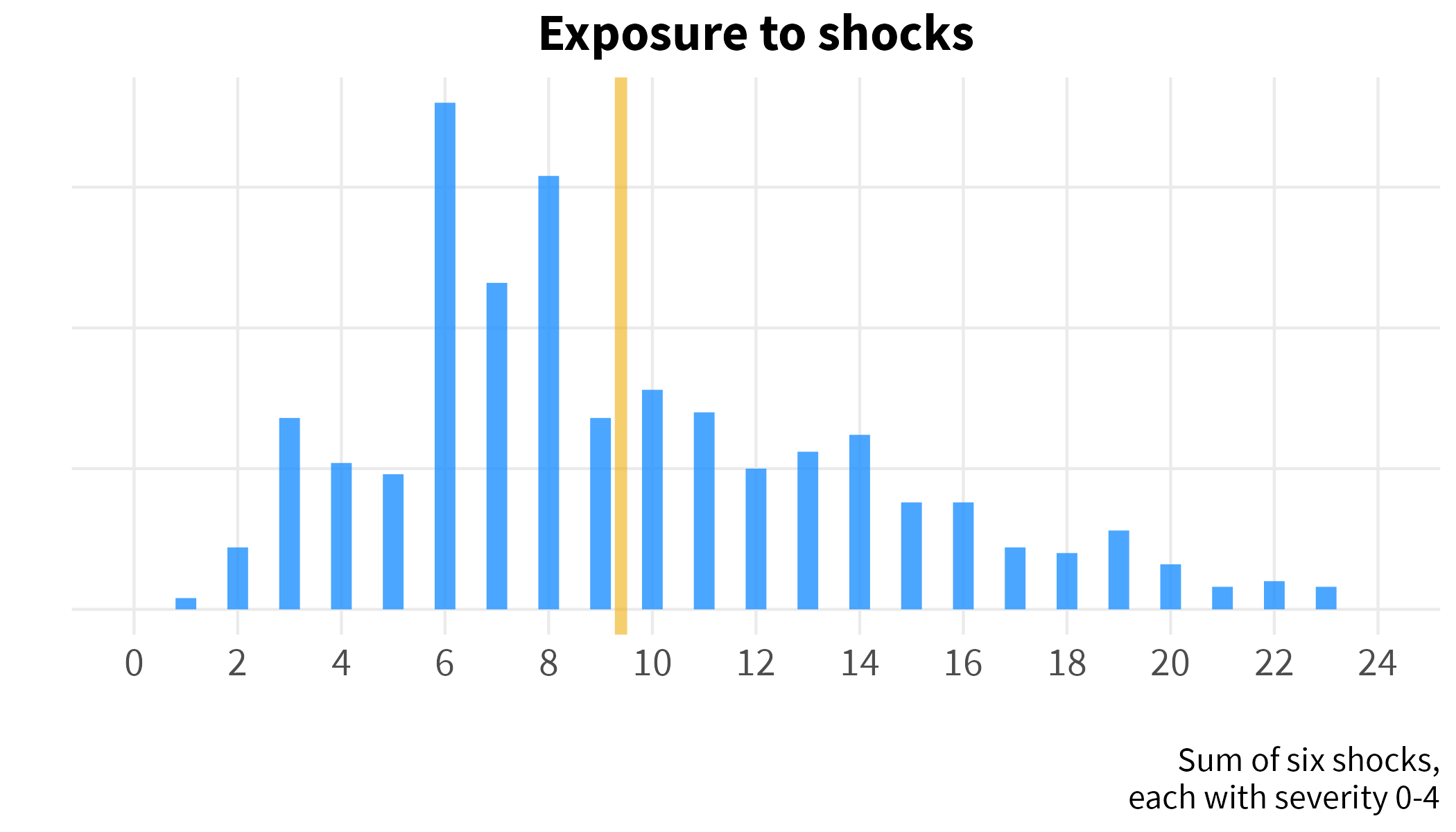
Household Shocks

Individual shocks

Code

shk <- read_csv(here("output/tables/Shock incidence.csv"),
                show_col_types=F)

shk_gt <- shk %>%
  dplyr::select(Shock, Percent) %>%
  mutate(Bar=Percent*100) %>%
  gt() %>%
  gt_plt_bar_pct(column=Bar, fill=usaid_blue, background=light_grey, scaled=T) %>%
  cols_width(3 ~ px(125)) %>%
  fmt_percent(2, decimals=0) %>%
  cols_label(Bar="")

shk_gt

Shock	Percent
Increase in food prices	98%
Drought	67%
Floods	50%
Theft	39%
Erosion	28%
Loss of land	17%

Total shock exposure

Code

include_graphics(here("output/viz/Exposure to shocks.png"))

Shock exposure, by county

Code

shocks_sev_cnty <- read_csv(here("output/tables/Shock severity county.csv"),
                            show_col_types = F)

shocks_sev_cnty_gt <- shocks_sev_cnty %>%
  dplyr::select(County, shocks_sev) %>%
  gt() %>%
  fmt_number(2, decimals=1) %>%
  cols_label(shocks_sev="Shock severity (0-24)")

shocks_sev_cnty_gt

County	Shock severity (0-24)
Akobo	13.8
Pibor	13.7
Jur River	9.9
Wau	7.0
Kapoeta North	6.4
Budi	5.5

Resilience

Resilience items

Code

resil <- read_csv(here("output/tables/Resilience binaries.csv"),
                  show_col_types=F)

resil_gt <- resil %>%
  dplyr::select(Resilience, Percent) %>%
  mutate(Bar=Percent*100) %>%
  gt() %>%
  gt_plt_bar_pct(column=Bar, fill=usaid_blue, background=light_grey, scaled=T) %>%
  cols_width(3 ~ px(125)) %>%
  fmt_percent(2, decimals=0) %>%
  cols_label(Bar="")

resil_gt

Resilience	Percent
Have learned from past shocks	71%
Can rely on family and friends	59%
Able to change livelihood to adapt to any shock	56%
Able to adapt to increased frequency or severity of shock	54%
Able to recover from shock	53%
Prepared for future shock	51%
Can rely on government support	40%
Able to access financial support	35%

Overall resilience

Resilience, by county

Development assistance

Natural resource management

Conflict

Community actions plans

Individual items

Code

emerg <- read_csv(here("output/tables/Community action plan binaries.csv"),
                  show_col_types = F)

emerg_gt <- emerg %>%
  dplyr::select(Item, Percent) %>%
  gt() %>%
  fmt_percent(2, decimals=0)

emerg_gt

Item	Percent
Community has emergency action plan	54%
Plan addresses at least one shock that affects community	89%
Plan is effective	19%

by county

Code

emerg_cnty <- read_csv(here("output/tables/Emergency action plans county.csv"),
                       show_col_types = F)

emerg_cnty_gt <- emerg_cnty %>%
  #dplyr::select(County, emerg_resc) %>%
  gt() %>%
  fmt_percent(2:4, decimals=0) %>%
  cols_label(emerg_plan="Emergency plan in place",
             emerg_targeted="Plan targeted to need",
             emerg_effective_bin="Plan effective")

emerg_cnty_gt

County	Emergency plan in place	Plan targeted to need	Plan effective
Akobo	64%	100%	3%
Budi	41%	90%	3%
Jur River	58%	71%	24%
Kapoeta North	32%	97%	12%
Pibor	67%	100%	40%
Wau	62%	79%	22%

Aspirations

Aspirations items

Code

asp <- read_csv(here("output/tables/Aspirations binaries.csv"),
                show_col_types = F)

asp_gt <- asp %>%
  dplyr::select(Aspiration, Percent) %>%
  mutate(Bar=Percent*100) %>%
  gt() %>%
  gt_plt_bar_pct(column=Bar, fill=usaid_blue, background=light_grey, scaled=T) %>%
  cols_width(3 ~ px(125)) %>%
  fmt_percent(2, decimals=0) %>%
  cols_label(Bar="")

asp_gt

Aspiration	Percent
Hopeful for children's future	91%
To be successful, above all one needs to work very hard	86%
Each person is primarily responsible for is/her success or failure in life	85%
Desire at least secondary school education for children	84%
Things turn out to be a matter of good or bad fortune (disagree)	22%
My experience in life has been that what is going to happen will happen (disagree)	16%

Overall aspirations

Aspirations, by county

Social norms

Acceptability of social and gender-based violence

Code

q812 <- read_csv(here("output/tables/q812.csv"),
                show_col_types = F)

q812_gt <- q812 %>%
  dplyr::select(gbv_lab, Percent) %>%
  mutate(Bar=Percent*100) %>%
  arrange(desc(Percent)) %>%
  gt() %>%
  gt_plt_bar_pct(column=Bar, fill=usaid_blue, background=light_grey, scaled=T) %>%
  cols_width(3 ~ px(125)) %>%
  fmt_percent(2, decimals=0) %>%
  cols_label(gbv_lab="Acceptability of violence",
             Bar="")

q812_gt

Acceptability of violence	Percent
Never	55%
Within a relationship, married	23%
To resolve dispute within the family	11%
In a time of conflict	5%
To resolve a dispute within a marriage	3%
Within a relationship, unmarried	2%
Other	1%

Acceptability of violence, by county

Code

gbv_accept_cnty <- read_csv(here("output/tables/Gender based violence acceptance county.csv"),
                            show_col_types = F)

gbv_accept_cnty_gt <- gbv_accept_cnty %>%
  dplyr::select(County, gbv_accept) %>%
  mutate(Bar=gbv_accept*100) %>%
  gt() %>%
  gt_plt_bar_pct(column=Bar, fill=usaid_blue, background=light_grey, scaled=T) %>%
  cols_width(3 ~ px(125)) %>%
  fmt_percent(2, decimals=0) %>%
  cols_label(gbv_accept="Acceptibility of gender-based violence",
             Bar="")

gbv_accept_cnty_gt

County	Acceptibility of gender-based violence
Wau	74%
Akobo	64%
Kapoeta North	41%
Pibor	41%
Budi	31%
Jur River	19%

Girls’ education

::: panel-tabset

Bride price

Acceptability of bride price

Code

bp <- read_csv(here("output/tables/Bride price binaries.csv"),
               show_col_types=F)

bp_gt <- bp %>%
  dplyr::select(Attitude, Percent) %>%
  mutate(Bar=Percent*100) %>%
  gt() %>%
  gt_plt_bar_pct(column=Bar, fill=usaid_blue, background=light_grey, scaled=T) %>%
  cols_width(3 ~ px(125)) %>%
  fmt_percent(2, decimals=0) %>%
  cols_label(Bar="")

bp_gt

Attitude	Percent
Bride price an important tradition	92%
Willing to accept a bride price for daughter in household	68%
Bride price an acceptable transaction	54%

Acceptability, by county

Code

bp_accept_cnty <- read_csv(here("output/tables/Bride price acceptance county.csv"),
                           show_col_types = F)

bp_accept_cnty_gt <- bp_accept_cnty %>%
  dplyr::select(County, bp_accept) %>%
  mutate(Bar=bp_accept*100) %>%
  gt() %>%
  gt_plt_bar_pct(column=Bar, fill=usaid_blue, background=light_grey, scaled=T) %>%
  cols_width(3 ~ px(125)) %>%
  fmt_percent(2, decimals=0) %>%
  cols_label(bp_accept="Acceptability of bride price",
             Bar="")

bp_accept_cnty_gt

County	Acceptability of bride price
Budi	94%
Pibor	84%
Kapoeta North	81%
Akobo	67%
Wau	46%
Jur River	36%

Trafficking in persons

Acceptability of trafficking

Code

traffic_accept <- read_csv(here("output/tables/q829 TIP.csv"),
                             show_col_types = F)

traffic_accept_gt <- traffic_accept %>%
  dplyr::select(traffic_labs, Percent) %>%
  mutate(Bar=Percent*100) %>%
  gt() %>%
  gt_plt_bar_pct(column=Bar, fill=usaid_blue, background=light_grey, scaled=T) %>%
  cols_width(3 ~ px(125)) %>%
  fmt_percent(2, decimals=0) %>%
  cols_label(traffic_labs="Trafficking Acceptability",
             Bar="")

traffic_accept_gt

Trafficking Acceptability	Percent
Revenge	6%
Money	0%
Have more children	0%
Never acceptable	94%

Code

TIP_agree <- read_csv(here("output/tables/TIP Binaries.csv"),
                      show_col_types = F)

TIP_gt <- TIP_agree %>%
  dplyr::select(TIP_agree, Percent) %>%
  mutate(Bar=Percent*100) %>%
  gt() %>%
  gt_plt_bar_pct(column=Bar, fill=usaid_blue, background=light_grey, scaled=T) %>%
  cols_width(3 ~ px(125)) %>%
  fmt_percent(2, decimals=0) %>%
  cols_label(TIP_agree="Acceptance of Trafficking",
              Bar="")

TIP_gt

Acceptance of Trafficking	Percent
To Get Cattle	11%
To Obtain A Wife	8%
To Get Land	5%

Acceptance of trafficking, by county

Code

TIP_accept_cnty <- read_csv(here("output/tables/TIP acceptance county.csv"),
                            show_col_types = F)

TIP_accept_cnty_gt <- TIP_accept_cnty %>%
  dplyr::select(County=county, Percent=traffic_accept) %>%
  mutate(Bar=Percent*100) %>%
  gt() %>%
  gt_plt_bar_pct(column=Bar, fill=usaid_blue, background=light_grey, scaled=T) %>%
  cols_width(3 ~ px(125)) %>%
  fmt_percent(2, decimals=0) %>%
  cols_label(#traffic_labs="Trafficking Acceptability",
             Bar="")

TIP_accept_cnty_gt

County	Percent
Akobo	31%
Pibor	3%
Budi	2%
Jur River	1%
Kapoeta North	0%
Wau	0%